

An Excel cell is nothing more than the intersection between a row and a column. The cells store the information of a reference, which can be of different types: text, numbers, monetary values, dates, functions, among others. The spreadsheet supports a multitude of references and operations. The cells are rectangular, although their size can be defined later by the user.
The user can also define the format of each cell by clicking on it with the right mouse button. When you do so, a context menu will be displayed, where you will see, among other things, the option to alter the formatting of the cells:
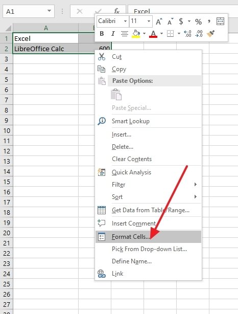 Cell format menu
If we click on it, the following window will appear, where we will be able to change the different formatting options of the cells in the following functions. In the Number tab (the first one that appears when opening the cell format) we can assign a category to each cell, ensuring that each data entered has a specific format:
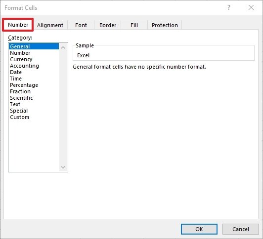 Number tab
The Alignment tab controls the arrangement of the text included in each cell:
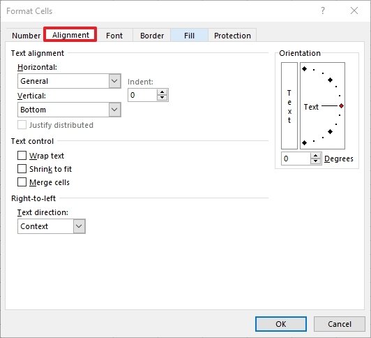 Alignment tab
In the Font tab, you can determine the type of font to represent the data that appear in each one. These fonts are common to all Office suite programs:
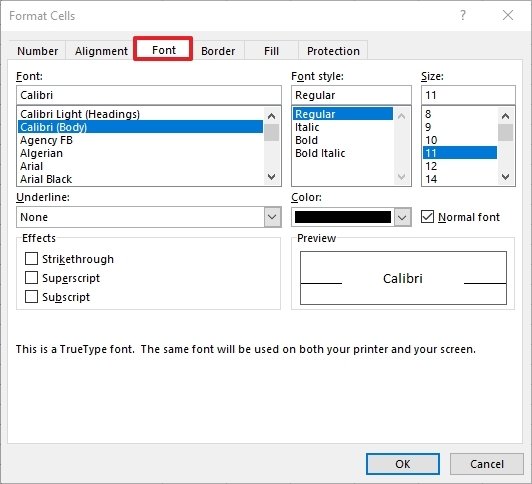 Font tab
In Border, we find what type of delimitation we are going to apply to each cell. This is a style adjustment, exactly the same as the previous one:
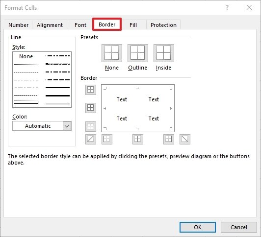 Border tab
In the Fill section, we can assign a particular background color to each cell or a set of cells, according to the needs of the user:
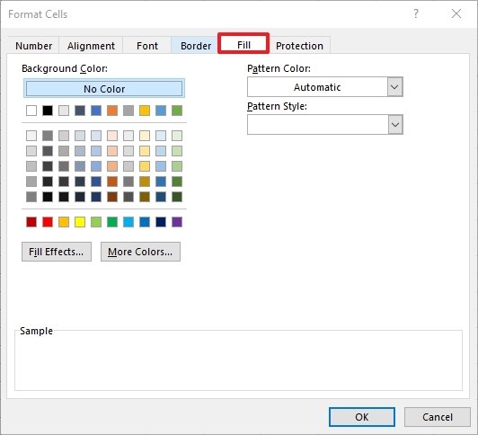 Fill tab
Finally, in the Protect section, we can block access to certain cells, or even hide them if we do not want other users to have access to their contents:
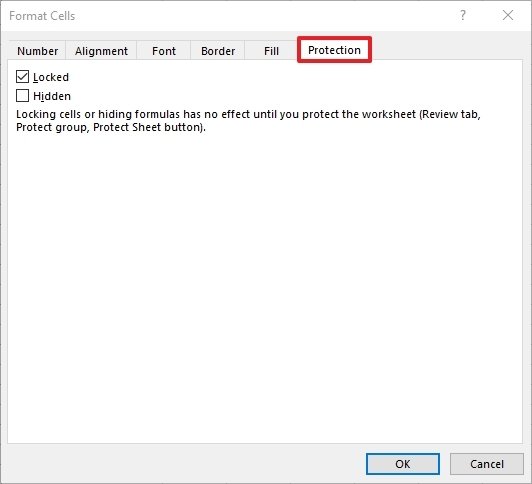 Protection tab
With this information in hand, everything will be much more logical and easier to understand.
